Breaking Down AI - Rainfall Prediction Using Machine Learning

AI is all around us now, it's moving so fast that at times it feels as if I'll never keep up. I'll try though. One common trend I've picked up on at work and in conversations with friends and family is that AI has become such a broad and mystical term it's almost meaningless. It could mean anything, but in reality it's been around us for decades. What is really new is truly advanced chat assistants like ChatGPT, Gemini, and Claude. For my friends family and colleagues I wanted to start a series on breaking down AI into it's constituent parts, the process of preparing data, selecting algorithms, training, evaluating, and many of the other steps that go into making these various AI services. So I'm starting this series where I will take a look at a single use case involving data science with a singular goal in mind. These will be like micro projects which may or may not work as intended, but will hopefully shed some light on the different ways AI is implemented.
Trying to explain every facet of the different processes involved in data science will be out of scope for this post, but I will try to explain what I understand and what I can as I go along.
For each blog post in this series there will be a corresponding Jupyter Labs notebook available, the notebook and dataset used for this post are here:
https://github.com/cskujawa/jupyter-notebooks/tree/main/ML/RainfallPredictions
Before diving into it, I want to talk a little about how AI is involved in predicting weather. Companies like the National Oceanic and Atmospheric Administration (NOAA) utilize sophisticated technologies and methodologies to make weather predictions. Some of which include machine learning like we will use in this blog post.
Neural Networks and Regression Models: Enhance specific aspects of forecasting, like precipitation or storm intensity predictions. -https://www.noaa.gov/ai/about
So, today I’m excited to share a project where I predicted daily rainfall (albeit inaccurately) using historical data and machine learning. This journey takes us through data preparation, visualization, model selection, training, and evaluation.
Preparing the Data
First, I loaded the dataset and began the process of cleaning it up. This involved checking for missing values, outliers, and any inconsistencies that might skew the results.
# Loading the Dataset
import pandas as pd

# Assuming the dataset is in a CSV file named 'rainfall_data.csv'
df = pd.read_csv('rainfall_data.csv')

# Display the first few rows of the dataframe
df.head()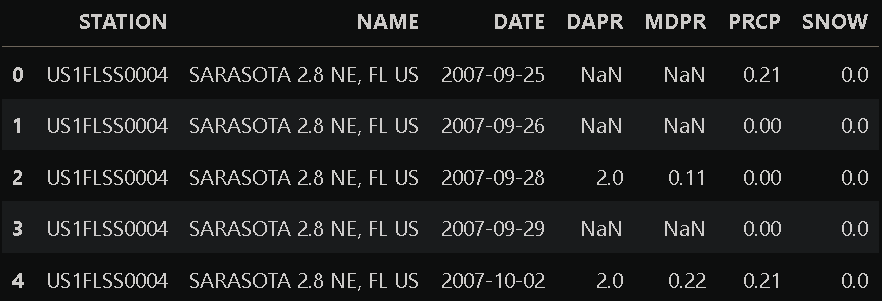
Cleaning the Data
I checked for missing values and filled them using forward fill to ensure there were no gaps that could affect the analysis.
# Checking for missing values
df.isnull().sum()

# Fill or drop missing values if necessary
df = df.ffill()

# Alternatively, you can use backward fill
# df = df.bfill()
Trimming Unnecessary Columns
Next, I removed any columns that weren’t relevant to the analysis, keeping only what was necessary.
# Keeping only relevant columns
# Assuming 'Date' and 'PRCP' are the relevant columns
df = df[['DATE', 'PRCP']]

# Renaming the 'PRCP' column to 'Rainfall'
df = df.rename(columns={'PRCP': 'Rainfall'})

# Display the first few rows of the cleaned dataframe
df.head()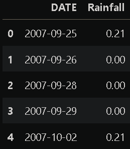
Exploring the Data
To understand the data better, I explored its structure and distribution.
# Summary statistics
df.describe()

# Checking the data types
df.info()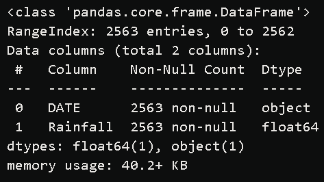
I had to do some additional cleaning to remove gaps in the timeline where there was no data, and I eventually ended up with this dataset.
Engineering Features
I created new features from the existing data to make it more informative for the model.
# Example: Extracting date-related features
df['DATE'] = pd.to_datetime(df['DATE'])
df['Year'] = df['DATE'].dt.year
df['Month'] = df['DATE'].dt.month
df['Day'] = df['DATE'].dt.day
Splitting the Data
I split the dataset into training and testing sets to evaluate the model’s performance accurately.
from sklearn.model_selection import train_test_split

# Define features and target variable
X = df[['Year', 'Month', 'Day']]
y = df['Rainfall']

# Split the data
X_train, X_test, y_train, y_test = train_test_split(X, y, test_size=0.2, random_state=42)
Choosing and Training Models
We will select a suitable machine learning model, train it on the training data, and evaluate its performance on the test data.
Linear Regression Model
A linear regression model is a statistical method used to model the relationship between a dependent variable and one or more independent variables. It assumes a linear relationship between the input variables (independent) and the output variable (dependent). The model attempts to find the best-fitting straight line (the regression line) that minimizes the difference (error) between the observed data points and the predicted values. This line is represented by the equation 𝑦=𝛽0+𝛽1𝑥+𝜖y=β0+β1x+ϵ, where 𝑦y is the dependent variable, 𝑥x is the independent variable, 𝛽0β0 is the y-intercept, 𝛽1β1 is the slope of the line, and 𝜖ϵ is the error term. Linear regression is widely used for prediction and forecasting in various fields such as economics, biology, engineering, and social sciences.
I started with a simple Linear Regression model to get a baseline performance.
from sklearn.linear_model import LinearRegression
from sklearn.metrics import mean_absolute_error, mean_squared_error

# Initialize the model
lr_model = LinearRegression()

# Train the model
lr_model.fit(X_train, y_train)

# Predictions
y_pred_lr = lr_model.predict(X_test)

# Evaluation
mae_lr = mean_absolute_error(y_test, y_pred_lr)
mse_lr = mean_squared_error(y_test, y_pred_lr)
Random Forest Model
A Random Forest model is an ensemble learning method used for classification and regression tasks. It constructs multiple decision trees during training and merges their results to produce a more accurate and stable prediction. Each tree in the forest is built using a random subset of the data and a random subset of the features, which helps to reduce overfitting and improve generalization. The final prediction is obtained by averaging the predictions of all the trees (for regression) or by majority voting (for classification). Random Forest models are known for their high accuracy, robustness to noise, and ability to handle large datasets with many features. They are widely used in various domains, including finance, healthcare, and image recognition.
Next, I tried a Random Forest model, known for its ability to handle more complex data patterns.
from sklearn.ensemble import RandomForestRegressor

# Initialize the model
rf_model = RandomForestRegressor(n_estimators=100, random_state=42)

# Train the model
rf_model.fit(X_train, y_train)

# Predictions
y_pred_rf = rf_model.predict(X_test)

# Evaluation
mae_rf = mean_absolute_error(y_test, y_pred_rf)
mse_rf = mean_squared_error(y_test, y_pred_rf)
Evaluating the Models
I compared the performance of both models using mean absolute error (MAE) and mean squared error (MSE).
# Model evaluation results
evaluation_results = {
    'Model': ['Linear Regression', 'Random Forest'],
    'MAE': [mae_lr, mae_rf],
    'MSE': [mse_lr, mse_rf]
}

# Display the evaluation results
pd.DataFrame(evaluation_results)
We compared the performance of two machine learning models: Linear Regression and Random Forest. The evaluation results for Mean Squared Error (MSE) were:
- Linear Regression: 0.1007
- Random Forest: 0.0901
The lower MSE value for the Random Forest model indicates that it performs better in predicting daily rainfall compared to the Linear Regression model.
Visualizing the Results
To see how well the models performed, I visualized the actual vs predicted rainfall values.
import matplotlib.pyplot as plt

# Plot actual vs predicted values for Linear Regression
plt.figure(figsize=(10, 5))
plt.plot(y_test.values, label='Actual')
plt.plot(y_pred_lr, label='Predicted - Linear Regression')
plt.legend()
plt.title('Actual vs Predicted Rainfall (Linear Regression)')
plt.show()

# Plot actual vs predicted values for Random Forest
plt.figure(figsize=(10, 5))
plt.plot(y_test.values, label='Actual')
plt.plot(y_pred_rf, label='Predicted - Random Forest')
plt.legend()
plt.title('Actual vs Predicted Rainfall (Random Forest)')
plt.show()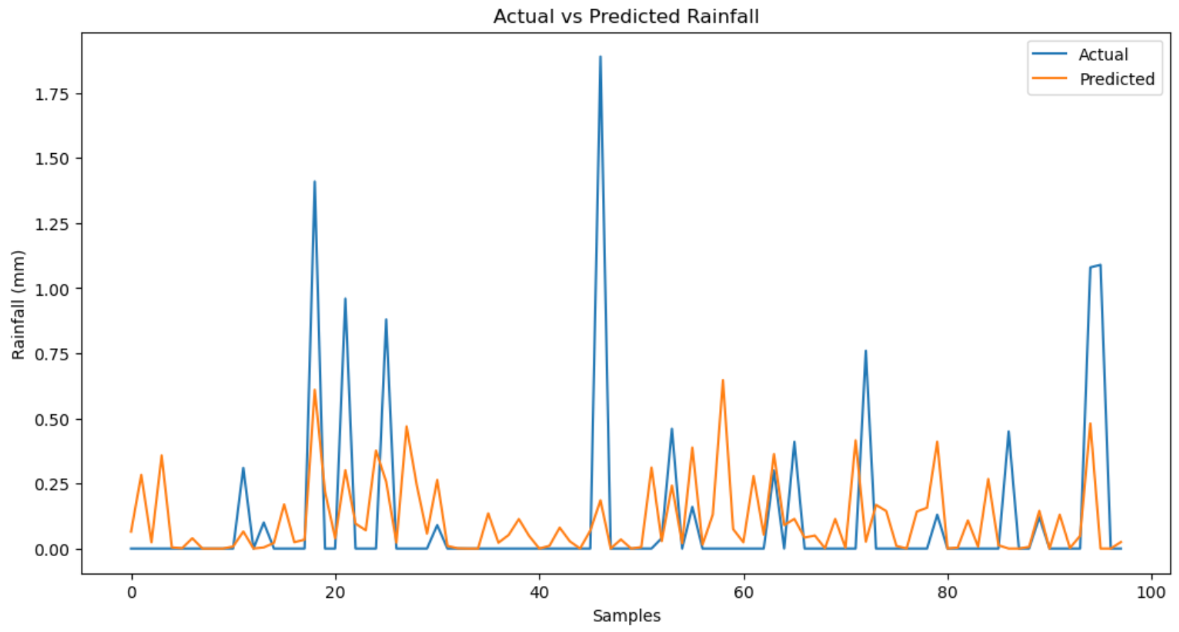
Reflections and Future Directions
Model Performance
The Random Forest model outperformed the Linear Regression model. It captured the trends and patterns in the data more effectively, as seen in the visualizations where predicted values closely followed the actual values.
Key Takeaways
- Model Selection: The Random Forest model is better suited for predicting daily rainfall in this dataset.
- Strengths: Its ability to handle non-linear relationships and interactions within the data.
- Areas for Improvement: Hyperparameter tuning, advanced models, and incorporating additional features like temperature and humidity.
Future Work
To further improve the model:
- Hyperparameter Tuning: Fine-tune the Random Forest parameters.
- Feature Engineering: Explore additional features such as weather conditions and seasonal indicators.
- Advanced Models: Experiment with LSTM or other time-series forecasting methods.
- Data Quality: Ensure a comprehensive and continuous dataset, possibly integrating more data sources.
Final Thoughts
This project highlighted the importance of choosing the right model and evaluating it thoroughly. The Random Forest model proved to be a reliable tool for predicting daily rainfall, but there is a lot of room for improvement.
By continuously refining the model and incorporating new data and techniques, we can enhance its accuracy and utility in real-world applications.
Thanks for following along on this journey. Stay tuned for more explorations into the world of data science and machine learning!